🎨 Seaborn for CA Professionals
Beautiful Statistical Charts with Minimal Code
Pre-requisite: Module 4 — Matplotlib
Estimated time: 4–5 hours
Session structure: Why Seaborn → What is Seaborn → Key Concepts → Hands-on → Dashboard
📋 Table of Contents
| Part | Section | Topic |
|---|---|---|
| Part 1: Why Seaborn? | 1 | What Matplotlib Cannot Do Easily |
| 2 | What is Seaborn? — History & Design | |
| Part 2: Fundamentals | 3 | Figure-level vs Axes-level Functions |
| 4 | Tidy Data — The Format Seaborn Expects | |
| 5 | Seaborn Themes & Palettes | |
| Part 3: Hands-on | 6 | Installing & Setup |
| 7 | Seaborn Themes (Hands-on) | |
| 8 | Distribution Plots — histplot & kdeplot | |
| 9 | Box Plot — Outlier Detection | |
| 10 | Violin Plot — Distribution Shape | |
| 11 | Bar & Count Plots | |
| 12 | Heatmap — Correlation Matrix | |
| 13 | Pair Plot — Multi-variable Exploration | |
| 14 | Scatter with Regression | |
| 15 | FacetGrid — Charts by Category | |
| 16 | Seaborn + Matplotlib Together | |
| Part 4: Practice | 17 | Practice Exercises |
Part 1: Why Seaborn?
Section 1: What Matplotlib Cannot Do Easily
You have just learned Matplotlib — Python's foundational chart library. Matplotlib gives you complete control. But "complete control" also means writing a lot of code for things that should be simple.
The verbosity problem
Imagine you want a box plot showing salary ranges across 5 departments, coloured by grade, with automatic outlier flagging.
In Matplotlib — approximately 25 lines:
fig, ax = plt.subplots(figsize=(12, 6))
departments = ['Finance', 'Operations', 'Sales', 'HR', 'IT']
grades = ['Junior', 'Mid', 'Senior', 'Lead']
colors = ['#4472C4', '#ED7D31', '#A9D18E', '#FF5757']
# ... manually group data by dept and grade
# ... manually draw each boxplot with ax.boxplot()
# ... manually set flierprops, whiskerprops, medianprops
# ... manually add legend
# ... manually format axes
In Seaborn — 1 line:
sns.boxplot(data=employees, x='Department', y='Annual_CTC', hue='Grade', palette='Set2')
What Seaborn adds over Matplotlib
| Task | Matplotlib | Seaborn |
|---|---|---|
| Grouped box plot | ~25 lines | 1 line |
| Correlation heatmap | ~20 lines | 2 lines |
| Distribution + KDE curve | ~10 lines | 1 line |
| Scatter with regression line | ~15 lines | 1 line |
| Multi-variable pair plot | ~30+ lines | 1 line |
| Category-split FacetGrid | ~20 lines | 3 lines |
Seaborn is NOT a replacement for Matplotlib
Seaborn builds on top of Matplotlib — every Seaborn chart is a Matplotlib chart underneath. This means:
- You can always use Matplotlib commands to customise a Seaborn chart
fig, ax = plt.subplots()still works — passax=axto Seaborn functionsplt.show(),fig.savefig()still save/display the chart
Think of Seaborn as Matplotlib with pre-built shortcuts for the most common statistical chart patterns.
Section 2: What is Seaborn? — History & Design
The Origin Story
In 2012, Michael Waskom was a graduate student at Stanford University (later a research scientist at NYU and Flatiron Institute). He was doing neuroscience research and found himself writing the same Matplotlib boilerplate code repeatedly for statistical visualizations.
He built a library of helper functions around Matplotlib and released it as Seaborn — named after the character Sam Seaborn from the TV show The West Wing.
"The goal of seaborn is to make a well-defined set of hard things easy."
— Michael Waskom
Seaborn was open-sourced in 2012. Today it has over 30 million downloads per month and is the standard library for statistical visualization in Python across academia, finance, and data science.
Design philosophy
Seaborn was designed around three principles:
- Dataset-oriented API: Pass the full DataFrame and column names — Seaborn figures out the groupings
- Statistical by default: Automatically computes means, confidence intervals, distributions
- Beautiful by default: Comes with tasteful colour palettes and clean themes out of the box
Where Seaborn fits
┌──────────────────────────────────────────────────────────────────────────┐
│    Seaborn — statistical visualization, beautiful defaults               │ ← You are here
├──────────────────────────────────────────────────────────────────────────┤
│    Matplotlib — complete, low-level chart control                        │ ← Module 4
├──────────────────────────────────────────────────────────────────────────┤
│    NumPy / Pandas — the data underneath                                  │ ← Modules 2 & 3
└──────────────────────────────────────────────────────────────────────────┘
Seaborn's strengths for CA professionals
| Analysis need | Seaborn chart |
|---|---|
| How are invoice amounts distributed? | histplot with KDE |
| Are there suspicious outliers in expenses? | boxplot — flags them automatically |
| Which financial ratios correlate? | heatmap on a correlation matrix |
| Do salaries differ by department? | violinplot or boxplot with hue |
| Is revenue growth statistically significant? | regplot with confidence band |
| Compare a metric across all departments × grade combinations | FacetGrid |
Part 2: Seaborn Fundamentals
Section 3: Figure-level vs Axes-level Functions
This is the most important conceptual distinction in Seaborn. Confusing these two types of functions is the most common source of errors.
Axes-level functions
Draw onto a specific Axes (subplot). These are the functions you will use most often.
| Function | Chart type |
|---|---|
sns.histplot() |
Histogram |
sns.kdeplot() |
Kernel density curve |
sns.boxplot() |
Box plot |
sns.violinplot() |
Violin plot |
sns.barplot() |
Bar chart with confidence intervals |
sns.countplot() |
Count bar chart |
sns.heatmap() |
Heatmap |
sns.regplot() |
Scatter with regression line |
sns.stripplot() |
Jittered strip plot |
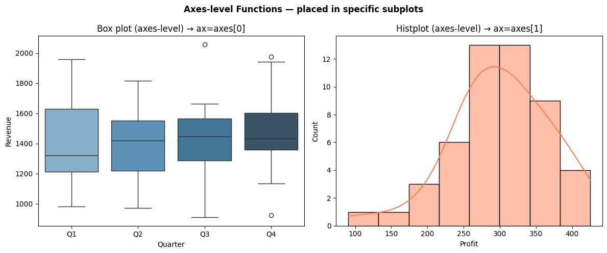
Key feature: Accept an ax= parameter — so you can place them inside Matplotlib subplots.
fig, axes = plt.subplots(1, 2)
sns.boxplot(data=df, x='Dept', y='Salary', ax=axes[0])   # goes in left subplot
sns.histplot(data=df, x='Amount', ax=axes[1])              # goes in right subplot
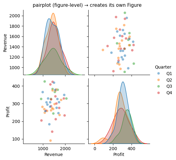
Figure-level functions
Create their own Figure and Axes internally. These return a special grid object, not a Matplotlib Axes.
| Function | What it creates |
|---|---|
sns.pairplot() |
Grid of scatter plots for all variable pairs |
sns.lmplot() |
Regression plot split by category |
sns.FacetGrid() |
Custom grid of any chart, split by category |
sns.catplot() |
Categorical plot (combines several axes-level functions) |
sns.displot() |
Distribution plot grid |
Key feature: Do NOT accept ax= — they manage their own Figure. You access the underlying Figure via .fig.
g = sns.pairplot(df)           # g is a PairGrid object
g.fig.suptitle('Pair Plot')    # access Figure like this
The rule
Use axes-level functions when you want to place a chart in a specific subplot of a larger dashboard.
Use figure-level functions when you want a standalone exploratory chart (pairplot, FacetGrid, lmplot).
import seaborn as sns
import matplotlib.pyplot as plt
import pandas as pd
import numpy as np

# --- Demonstrating axes-level vs figure-level ---

# Build a small sample
np.random.seed(42)
sample = pd.DataFrame({
    'Revenue': np.random.normal(1500, 300, 50),
    'Profit':  np.random.normal(300, 80, 50),
    'Quarter': np.random.choice(['Q1','Q2','Q3','Q4'], 50)
})

# AXES-LEVEL: can be placed in a subplot grid using ax=
fig, axes = plt.subplots(1, 2, figsize=(12, 5))
fig.suptitle('Axes-level Functions — placed in specific subplots', fontsize=12, fontweight='bold')

sns.boxplot(data=sample, x='Quarter', y='Revenue', ax=axes[0], palette='Blues_d')
axes[0].set_title('Box plot (axes-level) → ax=axes[0]')

sns.histplot(data=sample, x='Profit', kde=True, ax=axes[1], color='coral')
axes[1].set_title('Histplot (axes-level) → ax=axes[1]')

plt.tight_layout()
plt.show()

# FIGURE-LEVEL: creates its own figure, returns a Grid object
g = sns.pairplot(sample, hue='Quarter', height=2.5, plot_kws={'alpha': 0.5})
g.fig.suptitle('pairplot (figure-level) → creates its own Figure', y=1.02, fontsize=11)
plt.show()

print("Axes-level return type:", type(axes[0]))  # AxesSubplot
print("Figure-level return type:", type(g))       # PairGrid
/var/folders/kp/mytrwq8157q9s1tmw7r79fkm0000gn/T/ipykernel_11210/4191714505.py:20: FutureWarning:

Passing `palette` without assigning `hue` is deprecated and will be removed in v0.14.0. Assign the `x` variable to `hue` and set `legend=False` for the same effect.

  sns.boxplot(data=sample, x='Quarter', y='Revenue', ax=axes[0], palette='Blues_d')
Axes-level return type: <class 'matplotlib.axes._axes.Axes'>
Figure-level return type: <class 'seaborn.axisgrid.PairGrid'>
Section 4: Tidy Data — The Format Seaborn Expects
What is tidy data?
Seaborn is designed to work with tidy (long) format DataFrames. Understanding this format is essential — it determines how you pass data to Seaborn.
Tidy data rules (Hadley Wickham, 2014): 1. Each variable is in its own column 2. Each observation is in its own row 3. Each observational unit forms a table
Long format vs Wide format — the key distinction
Wide format (how we often store data in Excel):
Month  | Revenue  | COGS    | Net_Profit
-------|----------|---------|----------
Apr    | 1250000  | 750000  | 197000
May    | 1380000  | 828000  | 229000
Jun    | 1120000  | 672000  | 185000
Long (tidy) format (what Seaborn loves):
Month  | Metric      | Value
-------|-------------|--------
Apr    | Revenue     | 1250000
Apr    | COGS        | 750000
Apr    | Net_Profit  | 197000
May    | Revenue     | 1380000
...
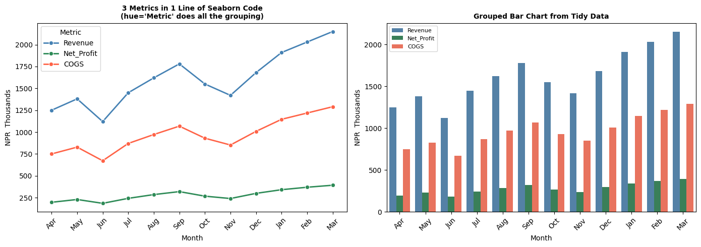
In the long format, Month and Metric are variables (columns), and Value is the observed value. Seaborn can now automatically group by Metric and colour bars differently — with a single hue='Metric' argument.
Converting between formats
| Direction | Pandas method |
|---|---|
| Wide → Long | pd.melt() |
| Long → Wide | df.pivot_table() or df.pivot() |
When to use which format
- Wide format: Pivot tables, Excel exports, DataFrames where each column is a distinct metric
- Long format: Seaborn charts, GroupBy operations, any analysis that treats metrics as a category
import pandas as pd
import seaborn as sns
import matplotlib.pyplot as plt

# --- Wide format (typical of what you'd import from Excel) ---
wide_df = pd.DataFrame({
    'Month':      ['Apr','May','Jun','Jul','Aug','Sep','Oct','Nov','Dec','Jan','Feb','Mar'],
    'Revenue':    [1250, 1380, 1120, 1450, 1620, 1780, 1550, 1420, 1680, 1910, 2030, 2150],
    'COGS':       [ 750,  828,  672,  870,  972, 1068,  930,  852, 1008, 1146, 1218, 1290],
    'Net_Profit': [ 197,  229,  185,  242,  285,  319,  267,  240,  299,  341,  369,  392],
})

print("Wide format (from Excel):")
print(wide_df.head(3))

# --- Convert to Long (tidy) format using pd.melt() ---
long_df = wide_df.melt(
    id_vars=['Month'],              # columns to keep as-is
    value_vars=['Revenue', 'COGS', 'Net_Profit'],   # columns to "unpivot"
    var_name='Metric',              # new column name for the former column headers
    value_name='Amount'             # new column name for the values
)

# Fix month order for charts (Apr → Mar, not alphabetical)
month_order = ['Apr','May','Jun','Jul','Aug','Sep','Oct','Nov','Dec','Jan','Feb','Mar']
long_df['Month'] = pd.Categorical(long_df['Month'], categories=month_order, ordered=True)
long_df = long_df.sort_values('Month')

print("\nLong (tidy) format after melt():")
print(long_df.head(9).to_string(index=False))

# --- Seaborn works beautifully with long format ---
fig, axes = plt.subplots(1, 2, figsize=(14, 5))

# One line draws all 3 metrics, coloured automatically
sns.lineplot(data=long_df, x='Month', y='Amount', hue='Metric', ax=axes[0],
             palette={'Revenue':'steelblue','COGS':'tomato','Net_Profit':'seagreen'},
             marker='o', linewidth=2)
axes[0].set_title('3 Metrics in 1 Line of Seaborn Code\n(hue=\'Metric\' does all the grouping)',
                  fontsize=10, fontweight='bold')
axes[0].set_ylabel('NPR  Thousands')
axes[0].tick_params(axis='x', rotation=45)

# Bar chart split by metric
sns.barplot(data=long_df, x='Month', y='Amount', hue='Metric', ax=axes[1],
            palette={'Revenue':'steelblue','COGS':'tomato','Net_Profit':'seagreen'})
axes[1].set_title('Grouped Bar Chart from Tidy Data', fontsize=10, fontweight='bold')
axes[1].set_ylabel('NPR  Thousands')
axes[1].tick_params(axis='x', rotation=45)
axes[1].legend(fontsize=8)

plt.tight_layout()
plt.show()
Wide format (from Excel):
  Month  Revenue  COGS  Net_Profit
0   Apr     1250   750         197
1   May     1380   828         229
2   Jun     1120   672         185

Long (tidy) format after melt():
Month     Metric  Amount
  Apr    Revenue    1250
  Apr Net_Profit     197
  Apr       COGS     750
  May    Revenue    1380
  May Net_Profit     229
  May       COGS     828
  Jun    Revenue    1120
  Jun Net_Profit     185
  Jun       COGS     672
Section 5: Seaborn Themes & Palettes
One of Seaborn's most valued features is its built-in themes and colour palettes. One line of code transforms the look of every chart in your notebook.
Built-in themes
| Theme | Look | Use when |
|---|---|---|
whitegrid |
White background, grey grid lines | Presentations, reports (most readable) |
darkgrid |
Dark background, grid lines | Technical reports, dark-mode screens |
white |
White background, no grid | Clean, minimal publications |
ticks |
White background, tick marks only | Academic papers |
dark |
Dark background, no grid | Rarely used |
Set globally (affects all subsequent charts):
sns.set_theme(style='whitegrid', palette='deep')
Set for one block only:
with sns.axes_style('darkgrid'):
    sns.histplot(...)   # only this chart uses darkgrid
Built-in colour palettes
| Palette | Type | Use when |
|---|---|---|
deep (default) |
Categorical | Different categories, no order |
Blues, Reds, Greens |
Sequential | Ordered data (low → high) |
RdYlGn |
Diverging | Data centred at zero (profit/loss, variance) |
colorblind |
Categorical | Presentations with accessibility needs |
husl |
Categorical | Many categories (> 6) |
rocket, mako |
Sequential | Modern, perceptually uniform |
Finance colour conventions in Seaborn
# For profit/loss charts — diverging palette centred at zero
sns.heatmap(data, cmap='RdYlGn', center=0)

# For variance (positive=good, negative=bad)
palette = {True: 'seagreen', False: 'tomato'}

# For categories (departments, expense heads)
sns.set_palette('deep')   # or 'colorblind' for accessible reports
Rule of thumb: Use
whitegridfor all classroom and client-facing charts. It's the cleanest, most universally readable theme.
Part 3: Hands-on with Seaborn
Section 6: Installing & Setup
# Install if needed
# !pip install seaborn matplotlib pandas numpy

import seaborn as sns
import matplotlib.pyplot as plt
import pandas as pd
import numpy as np

%matplotlib inline
plt.rcParams['figure.dpi'] = 100

print('Seaborn version:', sns.__version__)
print('Ready!')
Seaborn version: 0.13.2
Ready!
# ==== Build a rich financial dataset for this notebook ====
np.random.seed(42)

n = 200   # 200 employee records

departments = np.random.choice(['Finance', 'Operations', 'Sales', 'HR', 'IT'], n,
                                p=[0.20, 0.25, 0.30, 0.10, 0.15])
grades      = np.random.choice(['Junior', 'Mid', 'Senior', 'Lead'], n, p=[0.35, 0.30, 0.25, 0.10])

base_salary = {'Junior': 280000, 'Mid': 480000, 'Senior': 720000, 'Lead': 1080000}
salaries = np.array([base_salary[g] * np.random.uniform(0.85, 1.25) for g in grades])

experience  = np.array([{'Junior': 1.5, 'Mid': 4.0, 'Senior': 8.0, 'Lead': 12.0}[g] +
                         np.random.uniform(-1, 2) for g in grades]).clip(0, 20)
performance = np.clip(np.random.normal(3.2, 0.8, n), 1, 5).round(1)
bonus_pct   = np.clip(performance * 2.5 + np.random.uniform(-2, 3, n), 5, 25).round(1)
bonus_amt   = salaries * bonus_pct / 100

employees = pd.DataFrame({
    'Department': departments,
    'Grade':      grades,
    'Annual_CTC': salaries.round(0).astype(int),
    'Experience': experience.round(1),
    'Perf_Score': performance,
    'Bonus_Pct':  bonus_pct,
    'Bonus_Amt':  bonus_amt.round(0).astype(int),
})

# Invoice dataset
np.random.seed(7)
m = 300
invoice_df = pd.DataFrame({
    'Amount':    np.random.exponential(75000, m).clip(5000, 600000).round(-3).astype(int),
    'Category':  np.random.choice(['Materials', 'Services', 'Utilities', 'Travel', 'Misc'], m,
                                    p=[0.30, 0.25, 0.15, 0.20, 0.10]),
    'Month':     np.random.choice(['Apr','May','Jun','Jul','Aug','Sep',
                                    'Oct','Nov','Dec','Jan','Feb','Mar'], m),
    'VAT_Rate': np.random.choice([0, 13], m, p=[0.15, 0.85]),
    'Status':    np.random.choice(['Paid', 'Pending', 'Overdue'], m, p=[0.65, 0.25, 0.10]),
})

print(f'Employee dataset: {employees.shape[0]} records')
print(f'Invoice dataset:  {invoice_df.shape[0]} records')
print()
print(employees.head())
Employee dataset: 200 records
Invoice dataset:  300 records

   Department   Grade  Annual_CTC  Experience  Perf_Score  Bonus_Pct  \
0  Operations     Mid      427800         3.5         2.6        9.2
1          IT  Junior      339086         1.3         3.6       11.0
2       Sales  Junior      294588         1.0         4.7       14.7
3       Sales  Senior      850020         7.3         4.3       10.5
4     Finance     Mid      469450         3.4         4.5       13.1

   Bonus_Amt
0      39358
1      37299
2      43304
3      89252
4      61498
Section 7: Seaborn Themes
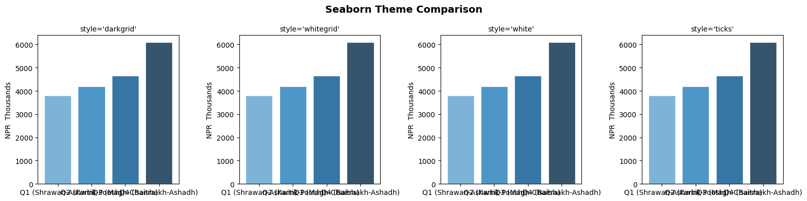
Seaborn gives you ready-made, professional themes. Just one line changes the look of all your charts.
# Available themes: darkgrid, whitegrid, dark, white, ticks
# Available palettes: deep, muted, bright, pastel, dark, colorblind, Blues, rocket, etc.

themes = ['darkgrid', 'whitegrid', 'white', 'ticks']

fig, axes = plt.subplots(1, 4, figsize=(16, 4))
fig.suptitle('Seaborn Theme Comparison', fontsize=14, fontweight='bold')

sample_x = ['Q1 (Shrawan-Ashwin)', 'Q2 (Kartik-Poush)', 'Q3 (Magh-Chaitra)', 'Q4 (Baishakh-Ashadh)']
sample_y = [3800, 4200, 4650, 6090]

for ax, theme in zip(axes, themes):
    with sns.axes_style(theme):
        ax.bar(sample_x, sample_y, color=sns.color_palette('Blues_d', 4))
        ax.set_title(f"style='{theme}'", fontsize=10)
        ax.set_ylabel('NPR  Thousands')

plt.tight_layout()
plt.show()

# Set a default theme for the rest of this notebook
sns.set_theme(style='whitegrid', palette='deep')
print("Default theme set to 'whitegrid' with 'deep' palette")
Default theme set to 'whitegrid' with 'deep' palette
Section 8: Distribution Plots — histplot & kdeplot
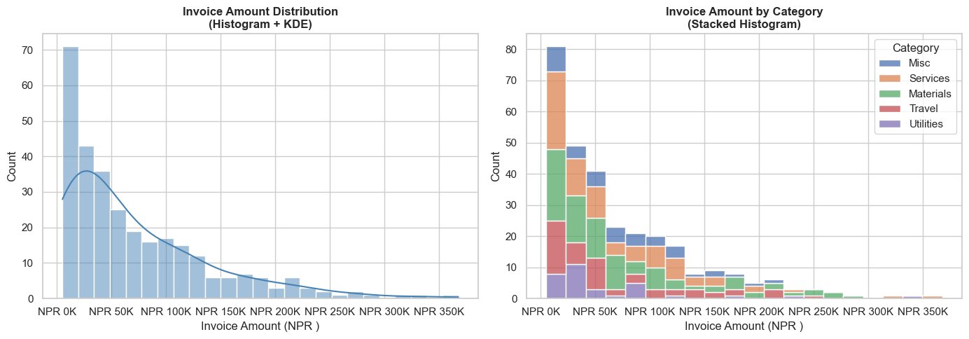
Distribution plots answer: "How are my values spread?"
For CA professionals: "Are most invoices small, or are large invoices common?"
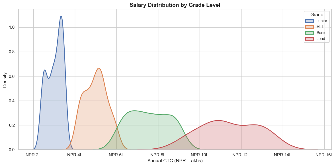
"Are salaries concentrated in one band or spread across many?"
# histplot — distribution of invoice amounts
fig, axes = plt.subplots(1, 2, figsize=(14, 5))

# Simple histogram
sns.histplot(data=invoice_df, x='Amount', bins=25, color='steelblue',
             kde=True, ax=axes[0])
axes[0].set_title('Invoice Amount Distribution\n(Histogram + KDE)', fontsize=12, fontweight='bold')
axes[0].set_xlabel('Invoice Amount (NPR )')
axes[0].xaxis.set_major_formatter(plt.FuncFormatter(lambda x, _: f'NPR {x/1000:.0f}K'))

# Histogram by Category
sns.histplot(data=invoice_df, x='Amount', hue='Category', bins=20,
             multiple='stack', ax=axes[1])
axes[1].set_title('Invoice Amount by Category\n(Stacked Histogram)', fontsize=12, fontweight='bold')
axes[1].set_xlabel('Invoice Amount (NPR )')
axes[1].xaxis.set_major_formatter(plt.FuncFormatter(lambda x, _: f'NPR {x/1000:.0f}K'))

plt.tight_layout()
plt.show()
# kdeplot — Salary distribution by Grade (smooth density curves)
fig, ax = plt.subplots(figsize=(12, 6))

for grade in ['Junior', 'Mid', 'Senior', 'Lead']:
    subset = employees[employees['Grade'] == grade]['Annual_CTC']
    sns.kdeplot(subset / 100000, label=grade, fill=True, alpha=0.25, linewidth=2, ax=ax)

ax.set_title('Salary Distribution by Grade Level', fontsize=14, fontweight='bold')
ax.set_xlabel('Annual CTC (NPR  Lakhs)')
ax.set_ylabel('Density')
ax.legend(title='Grade', fontsize=10)
ax.xaxis.set_major_formatter(plt.FuncFormatter(lambda x, _: f'NPR {x:.0f}L'))

plt.tight_layout()
plt.show()

print('Average CTC by Grade:')
print(employees.groupby('Grade')['Annual_CTC'].mean().sort_values().apply(lambda x: f'NPR {x/100000:.1f} Lakhs'))
Average CTC by Grade:
Grade
Junior     NPR 3.0 Lakhs
Mid        NPR 5.0 Lakhs
Senior     NPR 7.6 Lakhs
Lead      NPR 11.4 Lakhs
Name: Annual_CTC, dtype: object
Section 9: Box Plot — Outlier Detection
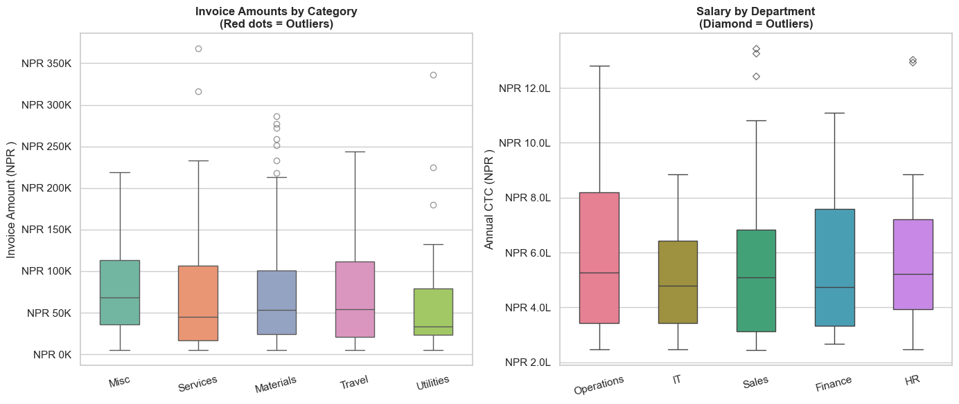
Box plots are one of the most important charts for auditors.
They show the spread of data and immediately highlight outliers — unusual values that may warrant investigation.
Reading a box plot:
         Outlier ●
              |
   Whisker ───┤ Upper fence (Q3 + 1.5×IQR)
              │
   Q3    ┌────┤ 75th percentile
         │    │
   Median├────┤ 50th percentile (orange line)
         │    │
   Q1    └────┤ 25th percentile
              │
   Whisker ───┤ Lower fence (Q1 - 1.5×IQR)
              |
         Outlier ●
# Box plot — Invoice amounts by category (flags outliers automatically)
fig, axes = plt.subplots(1, 2, figsize=(14, 6))

# Invoice amounts by expense category
sns.boxplot(data=invoice_df, x='Category', y='Amount',
            palette='Set2', ax=axes[0], width=0.5,
            flierprops=dict(marker='o', color='red', markersize=6, alpha=0.6))
axes[0].set_title('Invoice Amounts by Category\n(Red dots = Outliers)', fontsize=12, fontweight='bold')
axes[0].set_ylabel('Invoice Amount (NPR )')
axes[0].set_xlabel('')
axes[0].yaxis.set_major_formatter(plt.FuncFormatter(lambda y, _: f'NPR {y/1000:.0f}K'))
axes[0].tick_params(axis='x', rotation=15)

# Employee salary by department
sns.boxplot(data=employees, x='Department', y='Annual_CTC',
            palette='husl', ax=axes[1], width=0.5,
            flierprops=dict(marker='D', color='red', markersize=5, alpha=0.7))
axes[1].set_title('Salary by Department\n(Diamond = Outliers)', fontsize=12, fontweight='bold')
axes[1].set_ylabel('Annual CTC (NPR )')
axes[1].set_xlabel('')
axes[1].yaxis.set_major_formatter(plt.FuncFormatter(lambda y, _: f'NPR {y/100000:.1f}L'))
axes[1].tick_params(axis='x', rotation=15)

plt.tight_layout()
plt.show()
/var/folders/kp/mytrwq8157q9s1tmw7r79fkm0000gn/T/ipykernel_11210/888267004.py:5: FutureWarning:

Passing `palette` without assigning `hue` is deprecated and will be removed in v0.14.0. Assign the `x` variable to `hue` and set `legend=False` for the same effect.

  sns.boxplot(data=invoice_df, x='Category', y='Amount',
/var/folders/kp/mytrwq8157q9s1tmw7r79fkm0000gn/T/ipykernel_11210/888267004.py:15: FutureWarning:

Passing `palette` without assigning `hue` is deprecated and will be removed in v0.14.0. Assign the `x` variable to `hue` and set `legend=False` for the same effect.

  sns.boxplot(data=employees, x='Department', y='Annual_CTC',
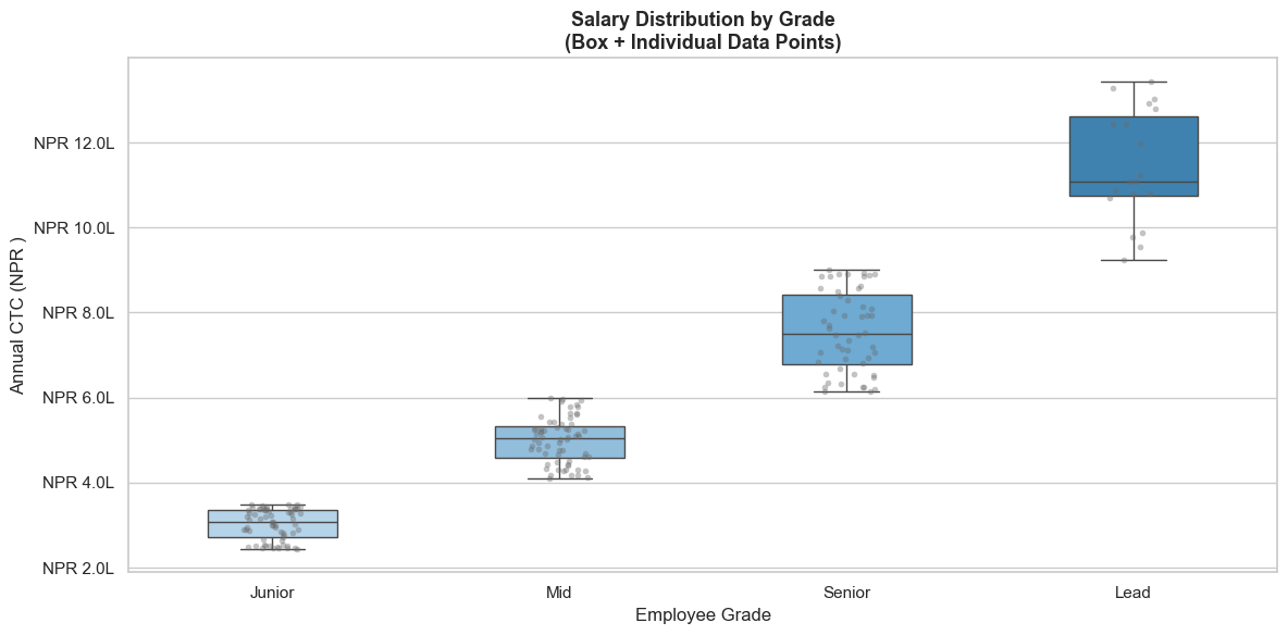
# Box plot with stripplot overlaid — shows individual data points
fig, ax = plt.subplots(figsize=(12, 6))

sns.boxplot(data=employees, x='Grade', y='Annual_CTC',
            order=['Junior', 'Mid', 'Senior', 'Lead'],
            palette=['#AED6F1','#85C1E9','#5DADE2','#2E86C1'],
            width=0.45, ax=ax,
            flierprops=dict(marker='', alpha=0))

sns.stripplot(data=employees, x='Grade', y='Annual_CTC',
              order=['Junior', 'Mid', 'Senior', 'Lead'],
              color='dimgray', alpha=0.4, size=4, jitter=True, ax=ax)

ax.set_title('Salary Distribution by Grade\n(Box + Individual Data Points)', fontsize=13, fontweight='bold')
ax.set_ylabel('Annual CTC (NPR )')
ax.set_xlabel('Employee Grade')
ax.yaxis.set_major_formatter(plt.FuncFormatter(lambda y, _: f'NPR {y/100000:.1f}L'))

plt.tight_layout()
plt.show()
/var/folders/kp/mytrwq8157q9s1tmw7r79fkm0000gn/T/ipykernel_11210/660531211.py:4: FutureWarning:

Passing `palette` without assigning `hue` is deprecated and will be removed in v0.14.0. Assign the `x` variable to `hue` and set `legend=False` for the same effect.

  sns.boxplot(data=employees, x='Grade', y='Annual_CTC',
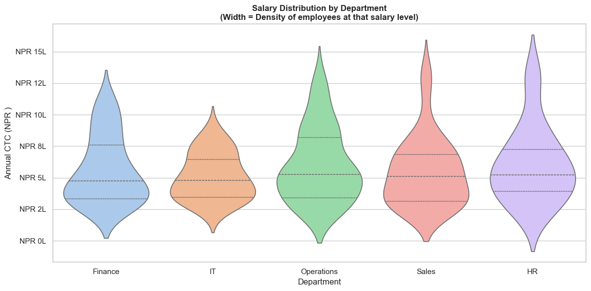
Section 10: Violin Plot — Distribution Shape by Category
A violin plot combines a box plot with a KDE — it shows both summary statistics AND the full distribution shape.
# Violin plot — salary distribution by department
fig, ax = plt.subplots(figsize=(12, 6))

sns.violinplot(data=employees, x='Department', y='Annual_CTC',
               palette='pastel', inner='quartile', ax=ax,
               order=['Finance', 'IT', 'Operations', 'Sales', 'HR'])

ax.set_title('Salary Distribution by Department\n(Width = Density of employees at that salary level)',
             fontsize=12, fontweight='bold')
ax.set_ylabel('Annual CTC (NPR )')
ax.set_xlabel('Department')
ax.yaxis.set_major_formatter(plt.FuncFormatter(lambda y, _: f'NPR {y/100000:.0f}L'))

plt.tight_layout()
plt.show()
/var/folders/kp/mytrwq8157q9s1tmw7r79fkm0000gn/T/ipykernel_11210/3679463453.py:4: FutureWarning:

Passing `palette` without assigning `hue` is deprecated and will be removed in v0.14.0. Assign the `x` variable to `hue` and set `legend=False` for the same effect.

  sns.violinplot(data=employees, x='Department', y='Annual_CTC',
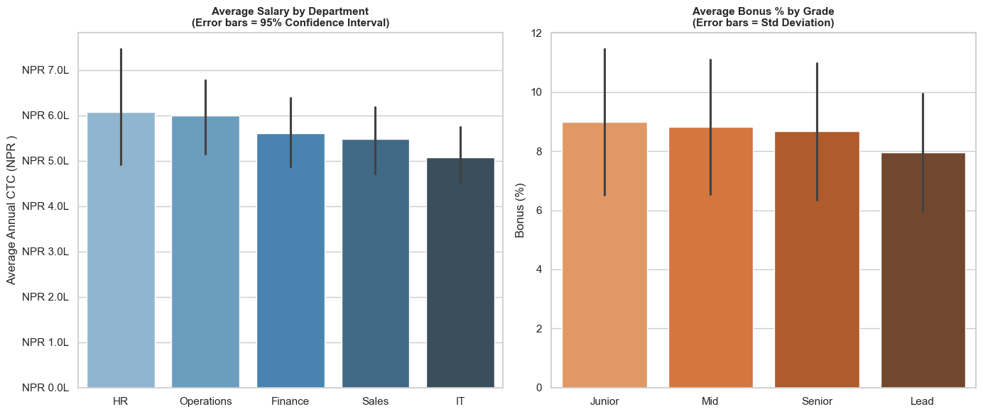
Section 11: Bar & Count Plots — Category Analysis
sns.barplot() automatically calculates and displays mean + confidence interval for each category — more insightful than plain bar charts.
# barplot — Average salary by Department (with confidence interval)
fig, axes = plt.subplots(1, 2, figsize=(14, 6))

# Average CTC by department
dept_order = employees.groupby('Department')['Annual_CTC'].mean().sort_values(ascending=False).index
sns.barplot(data=employees, x='Department', y='Annual_CTC',
            order=dept_order, palette='Blues_d',
            estimator='mean', errorbar='ci', ax=axes[0])
axes[0].set_title('Average Salary by Department\n(Error bars = 95% Confidence Interval)', fontsize=11, fontweight='bold')
axes[0].set_ylabel('Average Annual CTC (NPR )')
axes[0].set_xlabel('')
axes[0].yaxis.set_major_formatter(plt.FuncFormatter(lambda y, _: f'NPR {y/100000:.1f}L'))

# Average bonus by Grade
grade_order = ['Junior', 'Mid', 'Senior', 'Lead']
sns.barplot(data=employees, x='Grade', y='Bonus_Pct',
            order=grade_order, palette='Oranges_d',
            ax=axes[1], errorbar='sd')
axes[1].set_title('Average Bonus % by Grade\n(Error bars = Std Deviation)', fontsize=11, fontweight='bold')
axes[1].set_ylabel('Bonus (%)')
axes[1].set_xlabel('')

plt.tight_layout()
plt.show()
/var/folders/kp/mytrwq8157q9s1tmw7r79fkm0000gn/T/ipykernel_11210/3403452037.py:6: FutureWarning:

Passing `palette` without assigning `hue` is deprecated and will be removed in v0.14.0. Assign the `x` variable to `hue` and set `legend=False` for the same effect.

  sns.barplot(data=employees, x='Department', y='Annual_CTC',
/var/folders/kp/mytrwq8157q9s1tmw7r79fkm0000gn/T/ipykernel_11210/3403452037.py:16: FutureWarning:

Passing `palette` without assigning `hue` is deprecated and will be removed in v0.14.0. Assign the `x` variable to `hue` and set `legend=False` for the same effect.

  sns.barplot(data=employees, x='Grade', y='Bonus_Pct',
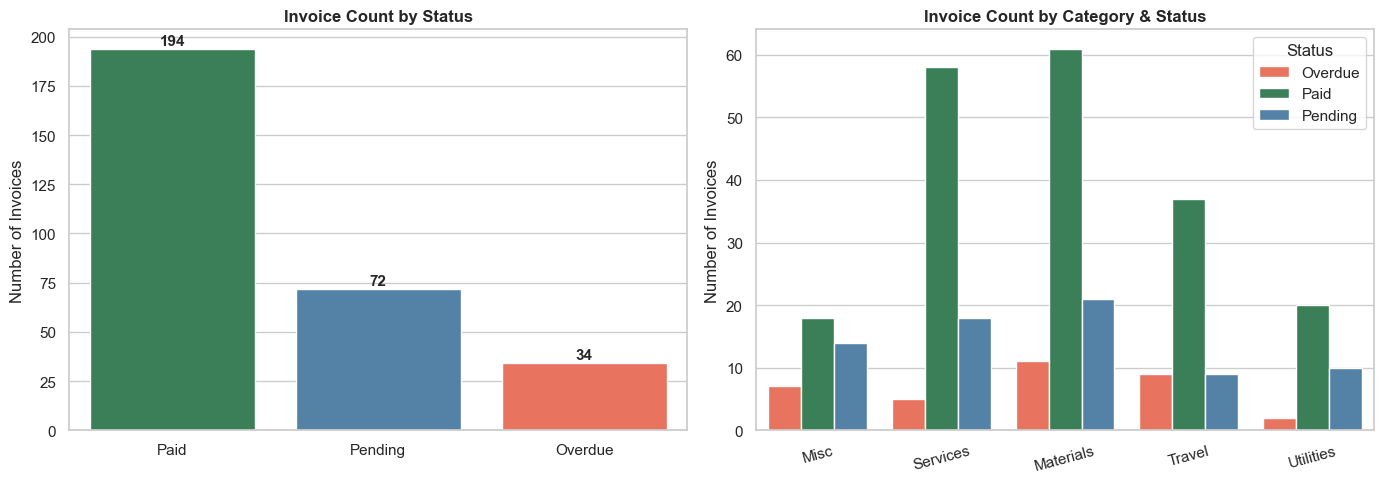
# countplot — how many invoices by status and category?
fig, axes = plt.subplots(1, 2, figsize=(14, 5))

# Count of invoices by status
sns.countplot(data=invoice_df, x='Status',
              palette={'Paid': 'seagreen', 'Pending': 'steelblue', 'Overdue': 'tomato'},
              order=['Paid', 'Pending', 'Overdue'], ax=axes[0])
axes[0].set_title('Invoice Count by Status', fontsize=12, fontweight='bold')
axes[0].set_ylabel('Number of Invoices')
axes[0].set_xlabel('')
for p in axes[0].patches:
    axes[0].annotate(f'{int(p.get_height())}', (p.get_x() + p.get_width()/2, p.get_height() + 2),
                     ha='center', fontsize=11, fontweight='bold')

# Count by category and status (hue)
sns.countplot(data=invoice_df, x='Category', hue='Status',
              palette={'Paid': 'seagreen', 'Pending': 'steelblue', 'Overdue': 'tomato'},
              ax=axes[1])
axes[1].set_title('Invoice Count by Category & Status', fontsize=12, fontweight='bold')
axes[1].set_ylabel('Number of Invoices')
axes[1].set_xlabel('')
axes[1].legend(title='Status')
axes[1].tick_params(axis='x', rotation=15)

plt.tight_layout()
plt.show()
/var/folders/kp/mytrwq8157q9s1tmw7r79fkm0000gn/T/ipykernel_11210/4118093210.py:5: FutureWarning:

Passing `palette` without assigning `hue` is deprecated and will be removed in v0.14.0. Assign the `x` variable to `hue` and set `legend=False` for the same effect.

  sns.countplot(data=invoice_df, x='Status',
Section 12: Heatmap — Correlation Matrix
A correlation heatmap shows how strongly pairs of variables are related.
In finance: "Does revenue growth correlate with headcount?" "Are salaries correlated with performance?"
Correlation values:
- +1.0 = Perfect positive relationship (as one rises, the other rises)
- 0.0 = No relationship
- -1.0 = Perfect negative relationship (as one rises, the other falls)
# Correlation heatmap for employee data
numeric_cols = employees[['Annual_CTC', 'Experience', 'Perf_Score', 'Bonus_Pct', 'Bonus_Amt']]
corr_matrix  = numeric_cols.corr().round(2)

fig, ax = plt.subplots(figsize=(9, 7))

sns.heatmap(
    corr_matrix,
    annot=True,           # Show correlation values in each cell
    fmt='.2f',            # 2 decimal places
    cmap='RdYlGn',        # Red (negative) → Yellow (zero) → Green (positive)
    center=0,             # Centre the colour scale at 0
    square=True,
    linewidths=1,
    linecolor='white',
    ax=ax,
    cbar_kws={'label': 'Correlation Coefficient'}
)

ax.set_title('Correlation Matrix — Employee Metrics', fontsize=14, fontweight='bold', pad=15)
ax.set_xticklabels(ax.get_xticklabels(), rotation=30, ha='right')

plt.tight_layout()
plt.show()

# Key insights
print('Key Insights from Correlation Matrix:')
r_exp   = corr_matrix.loc['Annual_CTC', 'Experience']
r_perf  = corr_matrix.loc['Annual_CTC', 'Perf_Score']
r_bns   = corr_matrix.loc['Bonus_Pct',  'Perf_Score']
lbl_exp  = 'Strong +ve' if abs(r_exp)  > 0.5 else 'Moderate'
lbl_perf = 'Strong +ve' if abs(r_perf) > 0.5 else 'Moderate'
print(f'  CTC vs Experience:  {r_exp}  — {lbl_exp}')
print(f'  Bonus% vs Perf:     {corr_matrix.loc["Bonus_Pct","Perf_Score"]}  — Performance drives bonus')
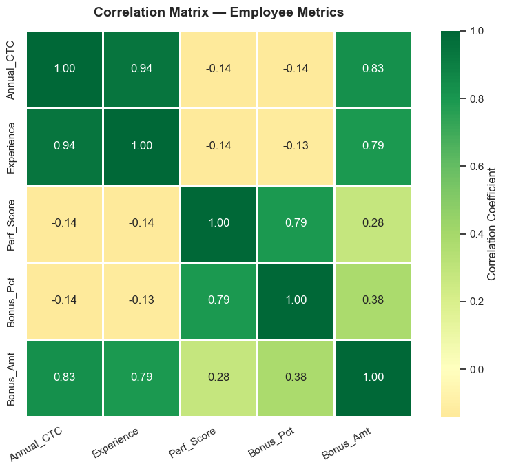
Key Insights from Correlation Matrix:
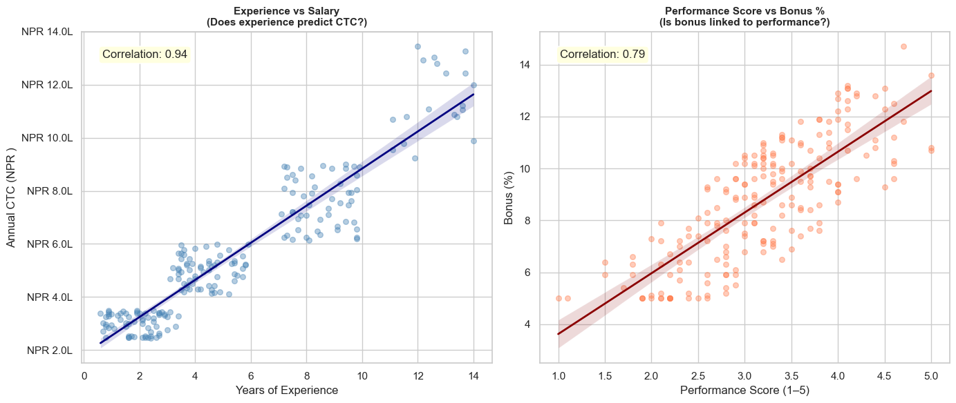
  CTC vs Experience:  0.94  — Strong +ve
  Bonus% vs Perf:     0.79  — Performance drives bonus
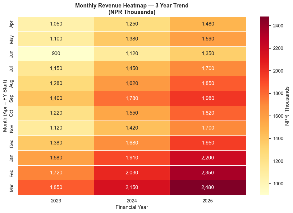
# Monthly revenue heatmap — very common in business analysis
# Simulate 3 years of monthly revenue data
np.random.seed(5)
years = [2023, 2024, 2025]
months_list = ['Apr', 'May', 'Jun', 'Jul', 'Aug', 'Sep', 'Oct', 'Nov', 'Dec', 'Jan', 'Feb', 'Mar']

base    = 1200
trend   = 80    # ~80K growth per month over years
monthly_rev = {
    2023: [1050, 1100, 900, 1150, 1280, 1400, 1220, 1120, 1380, 1580, 1720, 1850],
    2024: [1250, 1380, 1120, 1450, 1620, 1780, 1550, 1420, 1680, 1910, 2030, 2150],
    2025: [1480, 1590, 1350, 1700, 1850, 1980, 1820, 1700, 1950, 2200, 2350, 2480],
}

rev_df = pd.DataFrame(monthly_rev, index=months_list)

fig, ax = plt.subplots(figsize=(10, 7))

sns.heatmap(rev_df, annot=True, fmt=',.0f', cmap='YlOrRd',
            linewidths=0.5, linecolor='white', ax=ax,
            cbar_kws={'label': 'NPR  Thousands'})

ax.set_title('Monthly Revenue Heatmap — 3 Year Trend\n(NPR Thousands)', fontsize=13, fontweight='bold')
ax.set_xlabel('Financial Year')
ax.set_ylabel('Month (Apr = FY Start)')

plt.tight_layout()
plt.show()
Section 13: Pair Plot — Multi-variable Exploration
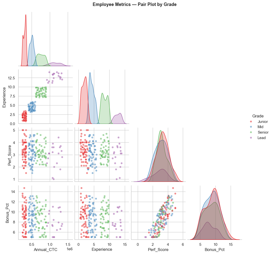
sns.pairplot() creates a grid of scatter plots for all pairs of numeric variables — ideal for initial data exploration. One line of code replaces many separate charts.
# Pair plot — all relationships in employee data at once
# Color-coded by Grade
pair_data = employees[['Annual_CTC', 'Experience', 'Perf_Score', 'Bonus_Pct', 'Grade']]

g = sns.pairplot(
    pair_data,
    hue='Grade',
    hue_order=['Junior', 'Mid', 'Senior', 'Lead'],
    palette='Set1',
    diag_kind='kde',     # Diagonal = KDE distribution
    plot_kws={'alpha': 0.5, 's': 30},
    corner=True          # Only lower triangle (avoids duplication)
)

g.fig.suptitle('Employee Metrics — Pair Plot by Grade', y=1.02, fontsize=13, fontweight='bold')
plt.show()
Section 14: Scatter with Regression — Relationships in Data
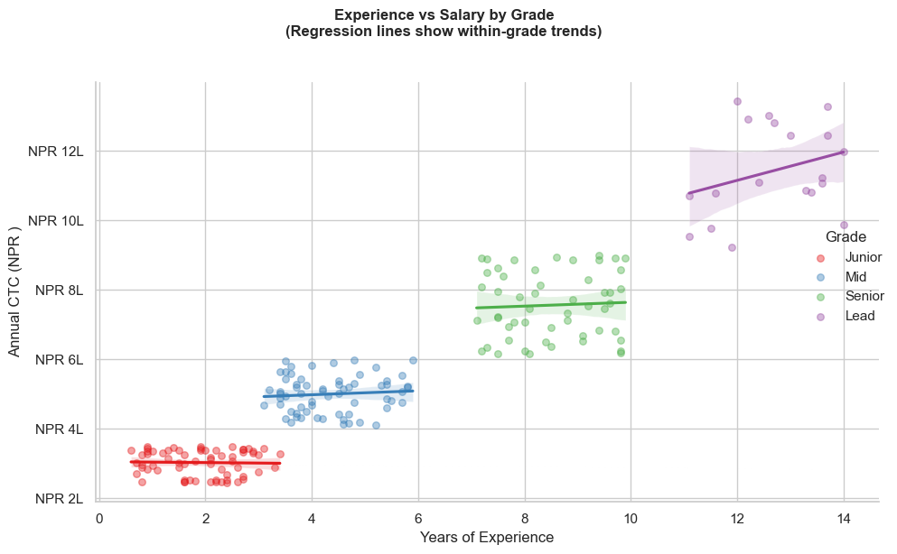
sns.regplot() and sns.lmplot() draw scatter plots with a regression line — shows the trend and whether two variables are truly related.
# regplot — does experience predict salary?
fig, axes = plt.subplots(1, 2, figsize=(14, 6))

# Plot 1: Experience vs CTC
sns.regplot(data=employees, x='Experience', y='Annual_CTC',
            scatter_kws={'alpha': 0.4, 's': 30, 'color': 'steelblue'},
            line_kws={'color': 'navy', 'linewidth': 2},
            ax=axes[0])
axes[0].set_title('Experience vs Salary\n(Does experience predict CTC?)', fontsize=11, fontweight='bold')
axes[0].set_xlabel('Years of Experience')
axes[0].set_ylabel('Annual CTC (NPR )')
axes[0].yaxis.set_major_formatter(plt.FuncFormatter(lambda y, _: f'NPR {y/100000:.1f}L'))

corr_exp_ctc = employees[['Experience', 'Annual_CTC']].corr().iloc[0, 1]
axes[0].text(0.05, 0.92, f'Correlation: {corr_exp_ctc:.2f}', transform=axes[0].transAxes,
             bbox=dict(boxstyle='round', facecolor='lightyellow'))

# Plot 2: Performance Score vs Bonus %
sns.regplot(data=employees, x='Perf_Score', y='Bonus_Pct',
            scatter_kws={'alpha': 0.4, 's': 30, 'color': 'coral'},
            line_kws={'color': 'darkred', 'linewidth': 2},
            ax=axes[1])
axes[1].set_title('Performance Score vs Bonus %\n(Is bonus linked to performance?)', fontsize=11, fontweight='bold')
axes[1].set_xlabel('Performance Score (1–5)')
axes[1].set_ylabel('Bonus (%)')

corr_perf_bonus = employees[['Perf_Score', 'Bonus_Pct']].corr().iloc[0, 1]
axes[1].text(0.05, 0.92, f'Correlation: {corr_perf_bonus:.2f}', transform=axes[1].transAxes,
             bbox=dict(boxstyle='round', facecolor='lightyellow'))

plt.tight_layout()
plt.show()
# lmplot — regression by subgroup (Grade)
g = sns.lmplot(
    data=employees,
    x='Experience',
    y='Annual_CTC',
    hue='Grade',
    hue_order=['Junior', 'Mid', 'Senior', 'Lead'],
    palette='Set1',
    scatter_kws={'alpha': 0.4, 's': 30},
    height=6, aspect=1.5
)

g.set_axis_labels('Years of Experience', 'Annual CTC (NPR )')
g.fig.suptitle('Experience vs Salary by Grade\n(Regression lines show within-grade trends)',
               y=1.02, fontsize=12, fontweight='bold')

# Format y-axis
for ax in g.axes.flat:
    ax.yaxis.set_major_formatter(plt.FuncFormatter(lambda y, _: f'NPR {y/100000:.0f}L'))

plt.tight_layout()
plt.show()
Section 15: FacetGrid — Charts by Category
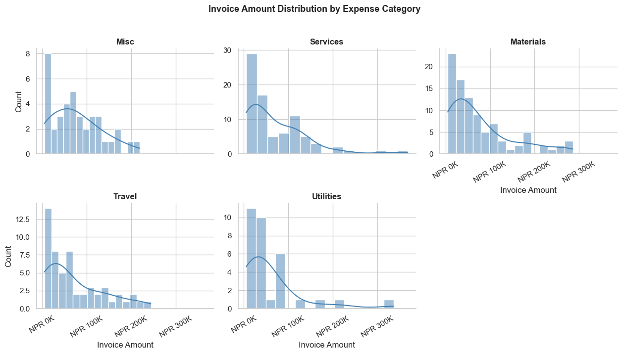
FacetGrid creates a grid of the same chart, split by a categorical variable. Like applying the same chart to each department, each quarter, etc.
# Invoice amount distribution — one histogram per expense category
g = sns.FacetGrid(
    invoice_df,
    col='Category',
    col_wrap=3,          # 3 charts per row
    height=3.5,
    aspect=1.2,
    sharey=False         # Allow different y-axis scales per chart
)

g.map(sns.histplot, 'Amount', bins=15, color='steelblue', kde=True)

for ax in g.axes.flat:
    ax.xaxis.set_major_formatter(plt.FuncFormatter(lambda x, _: f'NPR {x/1000:.0f}K'))
    ax.tick_params(axis='x', rotation=30)

g.set_axis_labels('Invoice Amount', 'Count')
g.set_titles(col_template='{col_name}', fontweight='bold')
g.fig.suptitle('Invoice Amount Distribution by Expense Category', y=1.02, fontsize=13, fontweight='bold')

plt.tight_layout()
plt.show()
Section 16: Seaborn + Matplotlib Together
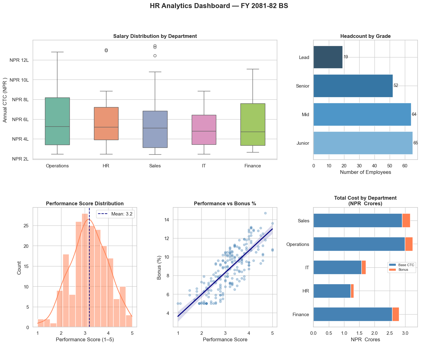
Seaborn and Matplotlib work together seamlessly. Use Seaborn for the chart, Matplotlib for fine-tuning.
# Comprehensive HR Analytics Dashboard
fig = plt.figure(figsize=(16, 12))
fig.suptitle('HR Analytics Dashboard — FY 2081-82 BS', fontsize=16, fontweight='bold', y=0.98)

# Layout using gridspec
gs = fig.add_gridspec(2, 3, hspace=0.4, wspace=0.35)

# Chart 1: Salary by Department (box plot)
ax1 = fig.add_subplot(gs[0, 0:2])
dept_order = employees.groupby('Department')['Annual_CTC'].median().sort_values(ascending=False).index
sns.boxplot(data=employees, x='Department', y='Annual_CTC',
            order=dept_order, palette='Set2', ax=ax1, width=0.5)
ax1.set_title('Salary Distribution by Department', fontweight='bold')
ax1.set_ylabel('Annual CTC (NPR )')
ax1.set_xlabel('')
ax1.yaxis.set_major_formatter(plt.FuncFormatter(lambda y, _: f'NPR {y/100000:.0f}L'))

# Chart 2: Headcount by Grade (count plot)
ax2 = fig.add_subplot(gs[0, 2])
grade_counts = employees['Grade'].value_counts().reindex(['Junior','Mid','Senior','Lead'])
ax2.barh(grade_counts.index, grade_counts.values,
         color=sns.color_palette('Blues_d', 4))
for i, v in enumerate(grade_counts.values):
    ax2.text(v + 0.5, i, str(v), va='center', fontsize=10)
ax2.set_title('Headcount by Grade', fontweight='bold')
ax2.set_xlabel('Number of Employees')

# Chart 3: Performance distribution
ax3 = fig.add_subplot(gs[1, 0])
sns.histplot(data=employees, x='Perf_Score', bins=15, kde=True, color='coral', ax=ax3)
ax3.axvline(employees['Perf_Score'].mean(), color='navy', linestyle='--',
             label=f"Mean: {employees['Perf_Score'].mean():.1f}")
ax3.set_title('Performance Score Distribution', fontweight='bold')
ax3.set_xlabel('Performance Score (1–5)')
ax3.legend()

# Chart 4: Bonus % vs Perf regression
ax4 = fig.add_subplot(gs[1, 1])
sns.regplot(data=employees, x='Perf_Score', y='Bonus_Pct',
            scatter_kws={'alpha': 0.35, 's': 25, 'color': 'steelblue'},
            line_kws={'color': 'navy'}, ax=ax4)
ax4.set_title('Performance vs Bonus %', fontweight='bold')
ax4.set_xlabel('Performance Score')
ax4.set_ylabel('Bonus (%)')

# Chart 5: Dept cost breakdown (stacked bar)
ax5 = fig.add_subplot(gs[1, 2])
dept_cost = employees.groupby('Department')[['Annual_CTC', 'Bonus_Amt']].sum() / 1e7  # In NPR  Crores
dept_cost.plot(kind='barh', stacked=True, ax=ax5,
               color=['steelblue', 'coral'], width=0.6)
ax5.set_title('Total Cost by Department\n(NPR  Crores)', fontweight='bold')
ax5.set_xlabel('NPR  Crores')
ax5.set_ylabel('')
ax5.legend(['Base CTC', 'Bonus'], fontsize=8)

plt.show()
/var/folders/kp/mytrwq8157q9s1tmw7r79fkm0000gn/T/ipykernel_11210/2995762040.py:11: FutureWarning:

Passing `palette` without assigning `hue` is deprecated and will be removed in v0.14.0. Assign the `x` variable to `hue` and set `legend=False` for the same effect.

  sns.boxplot(data=employees, x='Department', y='Annual_CTC',
Section 17: Practice Exercises
🏋️ Exercise 1 — Invoice Outlier Analysis
Using the invoice_df dataset:
1. Create a box plot showing invoice amounts for each VAT rate (0% exempt, 13% standard — Nepal IRD classification)
2. Identify and print the invoices that are statistical outliers (above Q3 + 1.5×IQR)
3. Create a heatmap showing average invoice amount by Category and Status
import seaborn as sns
import matplotlib.pyplot as plt
import pandas as pd
import numpy as np

# (Re-run the data setup cell at the top if invoice_df is not available)

# Write your analysis here
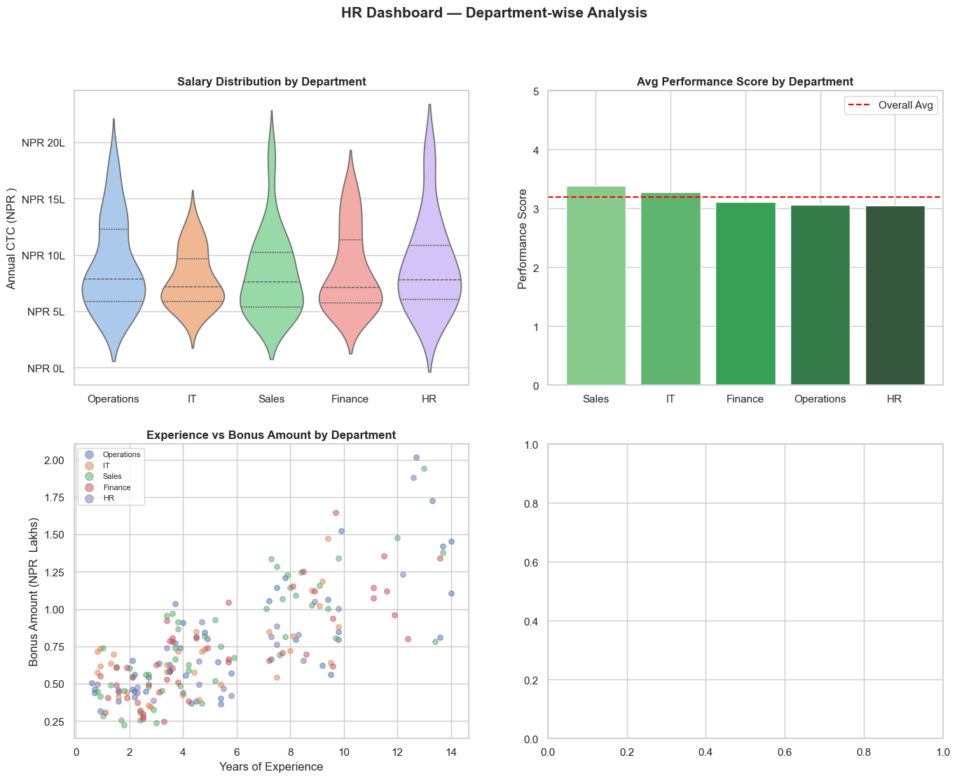
🏋️ Exercise 2 — Department-wise Financial Dashboard
Using the employees dataset, create a 2×2 subplot dashboard with:
1. Top-left: Violin plot of salary by department
2. Top-right: Bar plot of average performance score by department
3. Bottom-left: Scatter of Experience vs Bonus Amount, coloured by Department
4. Bottom-right: Heatmap of average salary by Department and Grade
Add appropriate titles and axis labels.
# Write your dashboard here
💡 Solutions
# SOLUTION — Exercise 1: Invoice Outlier Analysis
import seaborn as sns
import matplotlib.pyplot as plt
import pandas as pd
import numpy as np

# (Rebuild dataset if needed)
np.random.seed(7)
m = 300
invoice_df = pd.DataFrame({
    'Amount':   np.random.exponential(75000, m).clip(5000, 600000).round(-3).astype(int),
    'Category': np.random.choice(['Materials','Services','Utilities','Travel','Misc'], m, p=[0.30,0.25,0.15,0.20,0.10]),
    'VAT_Rate': np.random.choice([0, 13], m, p=[0.15, 0.85]),
    'Status':   np.random.choice(['Paid','Pending','Overdue'], m, p=[0.65, 0.25, 0.10]),
})

fig, axes = plt.subplots(1, 2, figsize=(15, 6))

# Box plot by GST rate
sns.boxplot(data=invoice_df, x='VAT_Rate', y='Amount', palette='coolwarm', ax=axes[0],
            flierprops=dict(marker='o', color='red', markersize=5, alpha=0.7))
axes[0].set_title('Invoice Amounts by GST Rate Slab\n(Red = Outliers)', fontweight='bold')
axes[0].set_xlabel('GST Rate (%)')
axes[0].set_ylabel('Invoice Amount (NPR )')
axes[0].yaxis.set_major_formatter(plt.FuncFormatter(lambda y, _: f'NPR {y/1000:.0f}K'))

# Heatmap: Avg Amount by Category & Status
pivot = invoice_df.pivot_table(values='Amount', index='Category', columns='Status', aggfunc='mean').round(0)
sns.heatmap(pivot, annot=True, fmt=',.0f', cmap='Blues', linewidths=0.5, ax=axes[1],
            cbar_kws={'label': 'Avg Invoice Amount (NPR )'})
axes[1].set_title('Avg Invoice Amount\nby Category & Status', fontweight='bold')

plt.tight_layout()
plt.show()

# Identify outliers
Q1, Q3 = invoice_df['Amount'].quantile([0.25, 0.75])
IQR    = Q3 - Q1
upper  = Q3 + 1.5 * IQR
outliers = invoice_df[invoice_df['Amount'] > upper]
print(f'Outlier threshold: NPR {upper:,.0f}')
print(f'Outlier count: {len(outliers)} ({len(outliers)/len(invoice_df)*100:.1f}% of invoices)')
print(f'Total outlier value: NPR {outliers["Amount"].sum():,.0f}')
/var/folders/kp/mytrwq8157q9s1tmw7r79fkm0000gn/T/ipykernel_11210/81329947.py:20: FutureWarning:

Passing `palette` without assigning `hue` is deprecated and will be removed in v0.14.0. Assign the `x` variable to `hue` and set `legend=False` for the same effect.

  sns.boxplot(data=invoice_df, x='VAT_Rate', y='Amount', palette='coolwarm', ax=axes[0],
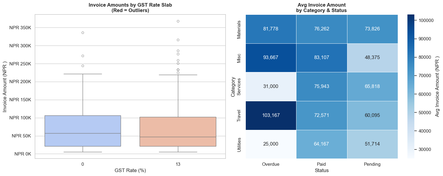
Outlier threshold: NPR 231,375
Outlier count: 11 (3.7% of invoices)
Total outlier value: NPR 3,075,000
# SOLUTION — Exercise 2: Department-wise Dashboard
import seaborn as sns, matplotlib.pyplot as plt, pandas as pd, numpy as np

# Rebuild employees if needed (copy from data setup cell)
np.random.seed(42)
n = 200
departments = np.random.choice(['Finance','Operations','Sales','HR','IT'], n, p=[0.20,0.25,0.30,0.10,0.15])
grades      = np.random.choice(['Junior','Mid','Senior','Lead'], n, p=[0.35,0.30,0.25,0.10])
base_salary = {'Junior':480000,'Mid':720000,'Senior':1080000,'Lead':1560000}
salaries    = np.array([base_salary[g] * np.random.uniform(0.85, 1.25) for g in grades])
experience  = np.array([{'Junior':1.5,'Mid':4.0,'Senior':8.0,'Lead':12.0}[g]+np.random.uniform(-1,2) for g in grades]).clip(0,20)
performance = np.clip(np.random.normal(3.2, 0.8, n), 1, 5).round(1)
bonus_pct   = np.clip(performance*2.5+np.random.uniform(-2,3,n), 5, 25).round(1)
bonus_amt   = salaries * bonus_pct / 100
employees   = pd.DataFrame({'Department':departments,'Grade':grades,'Annual_CTC':salaries.round(0).astype(int),
                             'Experience':experience.round(1),'Perf_Score':performance,
                             'Bonus_Pct':bonus_pct,'Bonus_Amt':bonus_amt.round(0).astype(int)})

fig, axes = plt.subplots(2, 2, figsize=(16, 12))
fig.suptitle('HR Dashboard — Department-wise Analysis', fontsize=15, fontweight='bold')

# 1. Violin — salary by department
sns.violinplot(data=employees, x='Department', y='Annual_CTC', palette='pastel', ax=axes[0,0], inner='quartile')
axes[0,0].set_title('Salary Distribution by Department', fontweight='bold')
axes[0,0].set_ylabel('Annual CTC (NPR )')
axes[0,0].set_xlabel('')
axes[0,0].yaxis.set_major_formatter(plt.FuncFormatter(lambda y,_: f'NPR {y/100000:.0f}L'))

# 2. Bar — avg performance score by dept
dept_perf = employees.groupby('Department')['Perf_Score'].mean().sort_values(ascending=False)
axes[0,1].bar(dept_perf.index, dept_perf.values, color=sns.color_palette('Greens_d', len(dept_perf)))
axes[0,1].axhline(employees['Perf_Score'].mean(), color='red', linestyle='--', linewidth=1.5, label='Overall Avg')
axes[0,1].set_title('Avg Performance Score by Department', fontweight='bold')
axes[0,1].set_ylabel('Performance Score')
axes[0,1].set_ylim(0, 5)
axes[0,1].legend()

# 3. Scatter — Experience vs Bonus
for dept in employees['Department'].unique():
    sub = employees[employees['Department'] == dept]
    axes[1,0].scatter(sub['Experience'], sub['Bonus_Amt']/100000, label=dept, alpha=0.5, s=30)
axes[1,0].set_title('Experience vs Bonus Amount by Department', fontweight='bold')
axes[1,0].set_xlabel('Years of Experience')
axes[1,0].set_ylabel('Bonus Amount (NPR  Lakhs)')
axes[1,0].legend(fontsize=8, markerscale=1.5)

# 4. Heatmap — avg salary by Dept × Grade
heat_data = employees.pivot_table(values='Annual_CTC', index='Department', columns='Grade',
                                   columns_sort=False,
                                   aggfunc='mean').reindex(columns=['Junior','Mid','Senior','Lead']) / 100000
sns.heatmap(heat_data.round(1), annot=True, fmt='.1f', cmap='YlOrRd', ax=axes[1,1],
            cbar_kws={'label': 'Avg CTC (NPR  Lakhs)'}, linewidths=0.5)
axes[1,1].set_title('Avg Salary (NPR L) by Dept × Grade', fontweight='bold')
axes[1,1].set_ylabel('')

plt.tight_layout()
plt.show()
/var/folders/kp/mytrwq8157q9s1tmw7r79fkm0000gn/T/ipykernel_11210/3553043638.py:23: FutureWarning:

Passing `palette` without assigning `hue` is deprecated and will be removed in v0.14.0. Assign the `x` variable to `hue` and set `legend=False` for the same effect.

  sns.violinplot(data=employees, x='Department', y='Annual_CTC', palette='pastel', ax=axes[0,0], inner='quartile')


---------------------------------------------------------------------------

TypeError                                 Traceback (most recent call last)

Cell In[23], line 48
     45 axes[1,0].legend(fontsize=8, markerscale=1.5)
     47 # 4. Heatmap — avg salary by Dept × Grade
---> 48 heat_data = employees.pivot_table(values='Annual_CTC', index='Department', columns='Grade',
     49                                    columns_sort=False,
     50                                    aggfunc='mean').reindex(columns=['Junior','Mid','Senior','Lead']) / 100000
     51 sns.heatmap(heat_data.round(1), annot=True, fmt='.1f', cmap='YlOrRd', ax=axes[1,1],
     52             cbar_kws={'label': 'Avg CTC (NPR  Lakhs)'}, linewidths=0.5)
     53 axes[1,1].set_title('Avg Salary (NPR L) by Dept × Grade', fontweight='bold')


TypeError: DataFrame.pivot_table() got an unexpected keyword argument 'columns_sort'
🎉 Module 5 Complete — And That's the Full Series!
What you've learned in this module
| Chart | When to use |
|---|---|
histplot / kdeplot |
Distribution of invoices, salaries, returns |
boxplot |
Outlier detection, salary ranges, audit flags |
violinplot |
Distribution shape by category |
barplot |
Mean comparison with confidence intervals |
countplot |
Frequency analysis by category |
heatmap |
Correlation, monthly trends, segment × category analysis |
pairplot |
Multi-variable exploration in one chart |
regplot / lmplot |
Trend and regression by group |
FacetGrid |
Same chart repeated by category |
🏆 Full Course Summary
| Module | Library | Key Skills |
|---|---|---|
| 1 | Python | Variables, data types, loops, functions |
| 2 | NumPy | Arrays, vectorized math, NPV/IRR |
| 3 | Pandas | DataFrames, GroupBy, merge, Excel I/O |
| 4 | Matplotlib | Line, bar, pie, histogram, dashboard |
| 5 | Seaborn | Statistical charts, heatmaps, outlier detection |
What's Next?
- Real project: Apply these skills to your own firm's data
- openpyxl / xlsxwriter: Create formatted Excel reports from Python
- reportlab / fpdf: Generate professional PDF reports automatically
- scikit-learn: Machine learning for fraud detection and risk scoring
- Streamlit / Dash: Build interactive financial dashboards
"Data is the new audit trail. Python is the new working paper."
Python for CA Professionals — Module 5: Seaborn
End of Introductory Series